Isa AlDoseri - Bahrain’s Solar & Wind Power Data 2022

Introduction

In this notebook, we shall take a look at solar and wind power output for the year 2022. The paper titled Evaluating solar and wind electricity production in the Kingdom of Bahrain to combat climate change, remarks on readings taken for the whole year, and has even sourced data for the weather conditions for the whole year (though this may seem unsubstantial at first considering they are monthly averages)

In this notebook, we will try to find correlations between the weather variables and the power-output in the dataset, and ultimately, find predictors we can use to predict solar/wind power. We will look at both power outputs separately.

Data Requirements

All the CSV files can be found in the data/ folder - solar_daily_2022.csv: Solar power output in KwH for each day of the year 2022 - wind_daily_2022.csv: Wind power output in KwH for each day of the year 2022 - triple_vars_monthly.csv: Humidity (%), Temperature (celsius) & Wind Speed (m/s) for each month of the year 2022 - manama.csv : Extended set of weather variables for each day of the year 2022, sourced from Visual Crossing

Import Packages & Setup

Code

# IMPORT PACKAGES
import os
import seaborn as sns
import matplotlib.pyplot as plt
import numpy as np # linear algebra
import pandas as pd # data processing, CSV file I/O (e.g. pd.read_csv)
from pathlib import Path

Code

# For the Kaggle Environment, please uncomment below
# kaggle_root = '/kaggle/input/bahrain-solar-research-2022' 
# root_path = !ls
data_path = Path('data/')

Load Target Variables (Solar + Wind Power Output)

Code

solar_file = data_path/'solar_daily_2022.csv'
solar = pd.read_csv(solar_file)
solar.date = pd.to_datetime(solar.date)
solar.info()

<class 'pandas.core.frame.DataFrame'>
RangeIndex: 365 entries, 0 to 364
Data columns (total 2 columns):
 #   Column  Non-Null Count  Dtype         
---  ------  --------------  -----         
 0   date    365 non-null    datetime64[ns]
 1   value   365 non-null    float64       
dtypes: datetime64[ns](1), float64(1)
memory usage: 5.8 KB

Code

wind = pd.read_csv(data_path/'wind_daily_2022.csv')
wind.date = pd.to_datetime(wind.date)
wind.info()
wind

<class 'pandas.core.frame.DataFrame'>
RangeIndex: 333 entries, 0 to 332
Data columns (total 2 columns):
 #   Column  Non-Null Count  Dtype         
---  ------  --------------  -----         
 0   date    333 non-null    datetime64[ns]
 1   value   333 non-null    float64       
dtypes: datetime64[ns](1), float64(1)
memory usage: 5.3 KB

	date	value
0	2022-01-31	79.75
1	2022-02-01	211.10
2	2022-02-02	195.53
3	2022-02-03	51.82
4	2022-02-04	83.44
...	...	...
328	2022-12-27	120.22
329	2022-12-28	926.98
330	2022-12-29	462.69
331	2022-12-30	273.46
332	2022-12-31	170.90

333 rows × 2 columns

Load Rest of the Data

Code

humidity_monthly = pd.read_csv(data_path/'humidity_percent_monthly_2022.csv')
temp_monthly = pd.read_csv(data_path/'temp_in_celcius_monthly_2022.csv')
wind_speed_monthly = pd.read_csv(data_path/'wind_speed_metre_per_second_monthly_2022.csv')
humidity_monthly.info()
temp_monthly.info()
wind_speed_monthly.info()

<class 'pandas.core.frame.DataFrame'>
RangeIndex: 12 entries, 0 to 11
Data columns (total 2 columns):
 #   Column  Non-Null Count  Dtype  
---  ------  --------------  -----  
 0   month   12 non-null     int64  
 1   value   12 non-null     float64
dtypes: float64(1), int64(1)
memory usage: 320.0 bytes
<class 'pandas.core.frame.DataFrame'>
RangeIndex: 12 entries, 0 to 11
Data columns (total 2 columns):
 #   Column  Non-Null Count  Dtype  
---  ------  --------------  -----  
 0   month   12 non-null     int64  
 1   value   12 non-null     float64
dtypes: float64(1), int64(1)
memory usage: 320.0 bytes
<class 'pandas.core.frame.DataFrame'>
RangeIndex: 12 entries, 0 to 11
Data columns (total 2 columns):
 #   Column  Non-Null Count  Dtype  
---  ------  --------------  -----  
 0   month   12 non-null     int64  
 1   value   12 non-null     float64
dtypes: float64(1), int64(1)
memory usage: 320.0 bytes

Plots

It always help to view plots of the dataset and how it varies in time.

Daily Power Output (Solar)

Code

plt.figure(figsize=(30, 7))
sns.lineplot(data=solar, x='date', y='value')

<AxesSubplot: xlabel='date', ylabel='value'>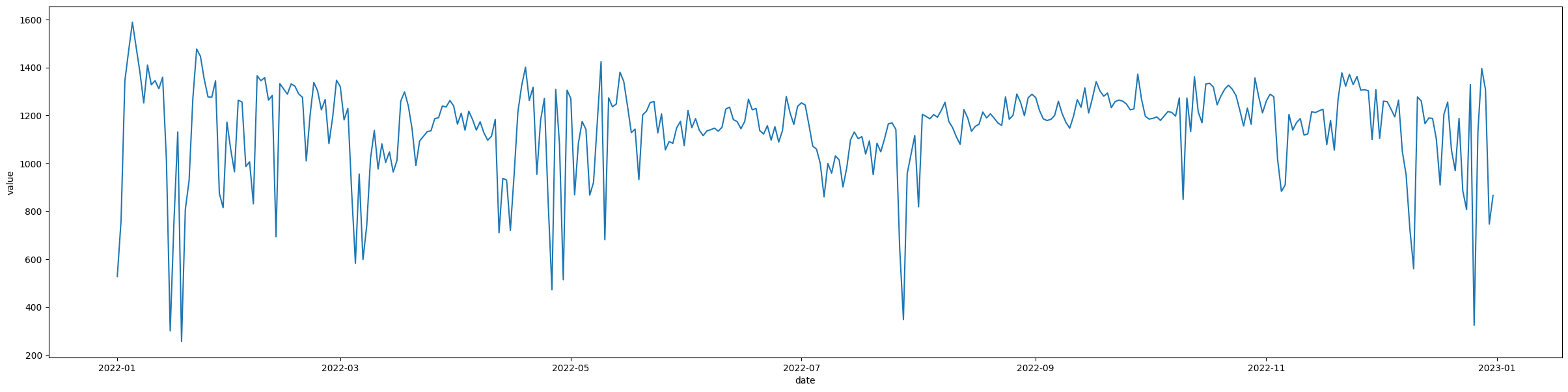

Daily Power Output (Wind)

Code

plt.figure(figsize=(30, 7))
sns.lineplot(data=wind, x='date', y='value')

<AxesSubplot: xlabel='date', ylabel='value'>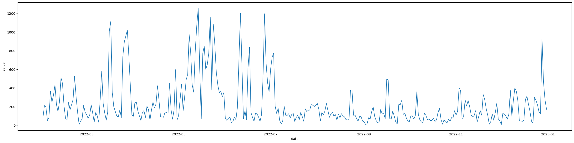

Weather Conditions (Monthly Basis)

Temperature (in Celcius)

Code

# plt.figure(figsize=(30, 7))
sns.lineplot(data=temp_monthly, x='month', y='value')

<AxesSubplot: xlabel='month', ylabel='value'>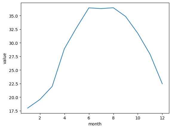

Wind Speed (m/s)

Code

sns.lineplot(data=wind_speed_monthly, x='month', y='value')

<AxesSubplot: xlabel='month', ylabel='value'>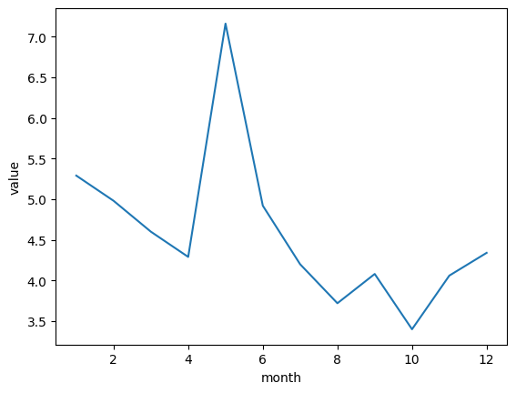

Humidity (%)

Code

# plt.figure(figsize=(30, 7))
sns.lineplot(data=humidity_monthly, x='month', y='value')

<AxesSubplot: xlabel='month', ylabel='value'>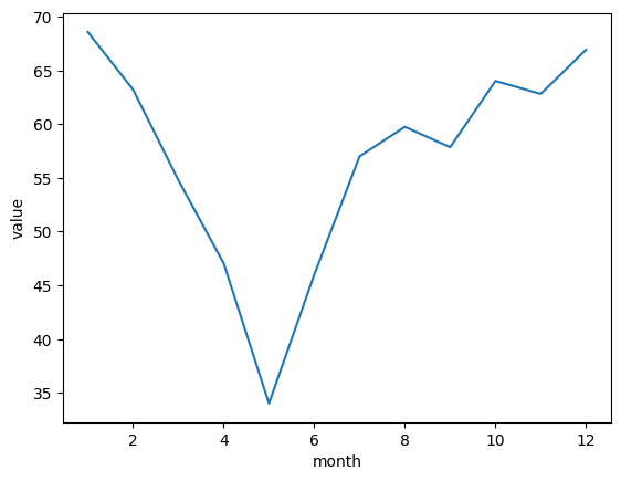

Combine Data

In this section, we will merge both the target variables and the features, to have one single dataframe to work with.

Code

wind_renamed = wind.rename(columns={'value': 'wind_power'})
solar_renamed = solar.rename(columns={'value': 'solar_power'})
target_data = wind_renamed.merge(solar_renamed, how='outer', on='date')
target_data = target_data.sort_values('date').reset_index(drop=True)
target_data

	date	wind_power	solar_power
0	2022-01-01	NaN	527.55
1	2022-01-02	NaN	762.18
2	2022-01-03	NaN	1343.82
3	2022-01-04	NaN	1469.36
4	2022-01-05	NaN	1588.27
...	...	...	...
360	2022-12-27	120.22	1132.27
361	2022-12-28	926.98	1395.73
362	2022-12-29	462.69	1307.64
363	2022-12-30	273.46	746.64
364	2022-12-31	170.90	865.91

365 rows × 3 columns

The wind power variable has missing values, let’s fill in the gap and see difference as different plots Wind power data with & without interpolation

Wind Power (Before Interpolation)

Code

plt.figure(figsize=(30, 7))
sns.lineplot(target_data, x='date', y='wind_power')

<AxesSubplot: xlabel='date', ylabel='wind_power'>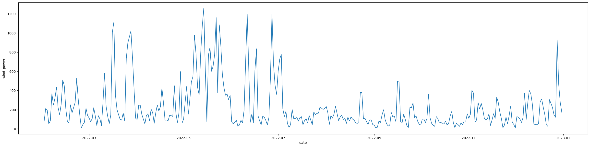

Wind Power (After Interpolation)

Code

target_data.wind_power = target_data.wind_power.interpolate(limit_direction='both')
plt.figure(figsize=(30, 7))
sns.lineplot(target_data, x='date', y='wind_power')

<AxesSubplot: xlabel='date', ylabel='wind_power'>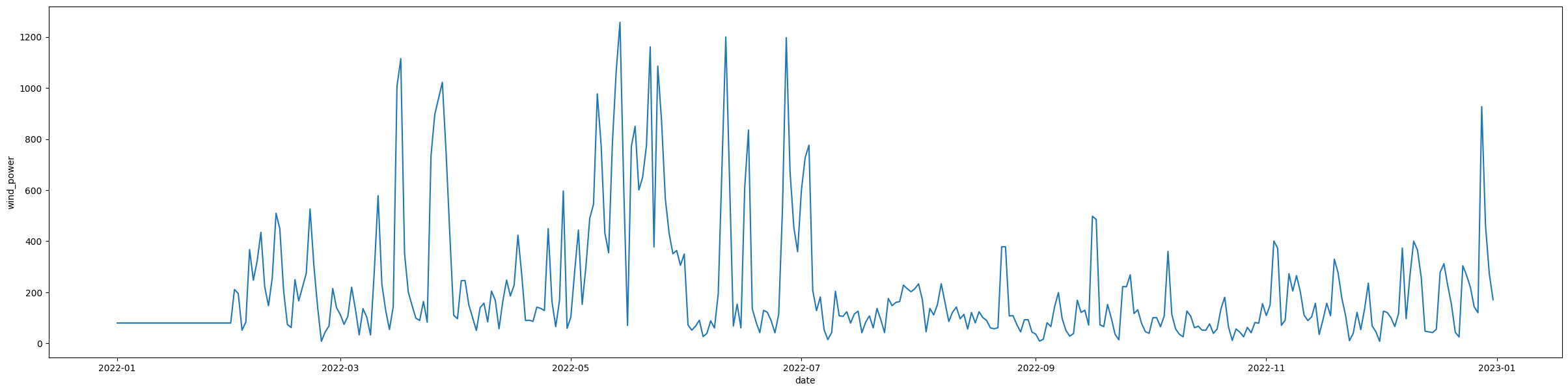

Correlation w/ Internal Data

What we will do now, is to find correlations between the weather variables and the power output (wind & solar). Considering that the weather conditions are only recorded once every month as opposed to the power output which is recorded on a daily basis; we will approximate the daily weather measurements with the month’s value i.e. if July had an average of 40 deg. celcius, then we will assume that every day of July had the same temperature.

Before that however, let’s combine these weather variables…

Code

target_data['month'] = target_data.date.dt.month
target_data

	date	wind_power	solar_power	month
0	2022-01-01	79.75	527.55	1
1	2022-01-02	79.75	762.18	1
2	2022-01-03	79.75	1343.82	1
3	2022-01-04	79.75	1469.36	1
4	2022-01-05	79.75	1588.27	1
...	...	...	...	...
360	2022-12-27	120.22	1132.27	12
361	2022-12-28	926.98	1395.73	12
362	2022-12-29	462.69	1307.64	12
363	2022-12-30	273.46	746.64	12
364	2022-12-31	170.90	865.91	12

365 rows × 4 columns

Code

wind_speed_monthly_renamed = wind_speed_monthly.rename(columns={'value': 'wind_speed'})
humidity_monthly_renamed = humidity_monthly.rename(columns={'value': 'humidity'})
temp_monthly_renamed = temp_monthly.rename(columns={'value': 'temp'})

_ = target_data.merge(wind_speed_monthly_renamed, on='month', how='inner')
_ = _.merge(humidity_monthly_renamed, on='month', how='inner')
_ = _.merge(temp_monthly_renamed, on='month', how='inner')


merged_all = _.copy()
merged_all

	date	wind_power	solar_power	month	wind_speed	humidity	temp
0	2022-01-01	79.75	527.55	1	5.29	68.57	17.99
1	2022-01-02	79.75	762.18	1	5.29	68.57	17.99
2	2022-01-03	79.75	1343.82	1	5.29	68.57	17.99
3	2022-01-04	79.75	1469.36	1	5.29	68.57	17.99
4	2022-01-05	79.75	1588.27	1	5.29	68.57	17.99
...	...	...	...	...	...	...	...
360	2022-12-27	120.22	1132.27	12	4.34	66.92	22.45
361	2022-12-28	926.98	1395.73	12	4.34	66.92	22.45
362	2022-12-29	462.69	1307.64	12	4.34	66.92	22.45
363	2022-12-30	273.46	746.64	12	4.34	66.92	22.45
364	2022-12-31	170.90	865.91	12	4.34	66.92	22.45

365 rows × 7 columns

Correlation Plot

Code

variables = ['wind_power', 'solar_power', 'wind_speed', 'humidity', 'temp']
corr = merged_all[variables].corr()
sns.heatmap(corr, annot=True)

<AxesSubplot: >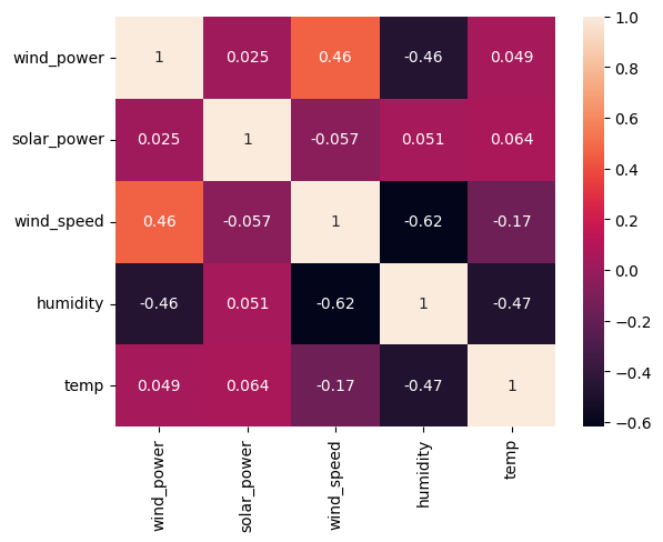

Results

For wind power, we can see humidity & wind speed have the highest correlations
For solar power, we don’t see any strong correlations
Notable features that correlate highly with one another are
- (temp, humidity)
- (wind_speed, humidity)

Sweetviz Package

The Sweetviz library is popular package to automate the analysis and display a competent report of the dataset. We will use this package with our original dataset, and with our extended set of features (manama.csv).

Code

import sweetviz as sv

Wind Power Report

Code

from IPython.display import display, Markdown

Code

analyze_report = sv.analyze([merged_all,'Wind Power Report'], 'wind_power')
filepath = 'reports/wind_power_internal_data.html'
analyze_report.show_html(filepath=filepath, layout='vertical', open_browser=False)
display(Markdown(f'**To view the report, [CLICK HERE]({filepath})**'))

Feature: wind_power (TARGET)                 |█▎        | [ 12%]   00:00 -> (00:00 left)Done! Use 'show' commands to display/save.   |██████████| [100%]   00:00 -> (00:00 left)

Report reports/wind_power_internal_data.html was generated.

To view the report, CLICK HERE

Conclusion

We can tell from this report, that there are a few variables, mainly wind_speed and humidity that corrleate highly with wind_power. We can use these as predictors

Solar Power Report

Code

analyze_report = sv.analyze([merged_all,'Solar Power Report'], 'solar_power')
filepath = 'reports/solar_power_internal_data.html'
analyze_report.show_html(filepath=filepath, layout='vertical', open_browser=False)
display(Markdown(f'**To view the report, [CLICK HERE]({filepath})**'))

Done! Use 'show' commands to display/save.   |██████████| [100%]   00:00 -> (00:00 left)

Report reports/solar_power_internal_data.html was generated.

To view the report, CLICK HERE

Conclusion

No suitable predictors can be found for solar_power. We don’t attempt to build a model around it.

Load Extended Weather Data

Code

external_weather_df = pd.read_csv(data_path/'manama.csv')
external_weather_df.rename(columns={'windspeed': 'wind_speed', 'datetime': 'date'}, inplace=True)
external_weather_df.date = pd.to_datetime(external_weather_df.date)
external_weather_df.info()

<class 'pandas.core.frame.DataFrame'>
RangeIndex: 365 entries, 0 to 364
Data columns (total 33 columns):
 #   Column            Non-Null Count  Dtype         
---  ------            --------------  -----         
 0   name              365 non-null    object        
 1   date              365 non-null    datetime64[ns]
 2   tempmax           365 non-null    float64       
 3   tempmin           365 non-null    float64       
 4   temp              365 non-null    float64       
 5   feelslikemax      365 non-null    float64       
 6   feelslikemin      365 non-null    float64       
 7   feelslike         365 non-null    float64       
 8   dew               365 non-null    float64       
 9   humidity          365 non-null    float64       
 10  precip            365 non-null    float64       
 11  precipprob        365 non-null    int64         
 12  precipcover       365 non-null    float64       
 13  preciptype        26 non-null     object        
 14  snow              351 non-null    float64       
 15  snowdepth         1 non-null      float64       
 16  windgust          356 non-null    float64       
 17  wind_speed        365 non-null    float64       
 18  winddir           365 non-null    float64       
 19  sealevelpressure  365 non-null    float64       
 20  cloudcover        365 non-null    float64       
 21  visibility        365 non-null    float64       
 22  solarradiation    365 non-null    float64       
 23  solarenergy       365 non-null    float64       
 24  uvindex           365 non-null    int64         
 25  severerisk        356 non-null    float64       
 26  sunrise           365 non-null    object        
 27  sunset            365 non-null    object        
 28  moonphase         365 non-null    float64       
 29  conditions        365 non-null    object        
 30  description       365 non-null    object        
 31  icon              365 non-null    object        
 32  stations          365 non-null    object        
dtypes: datetime64[ns](1), float64(22), int64(2), object(8)
memory usage: 94.2+ KB

Code

external_weather_df.columns

Index(['name', 'date', 'tempmax', 'tempmin', 'temp', 'feelslikemax',
       'feelslikemin', 'feelslike', 'dew', 'humidity', 'precip', 'precipprob',
       'precipcover', 'preciptype', 'snow', 'snowdepth', 'windgust',
       'wind_speed', 'winddir', 'sealevelpressure', 'cloudcover', 'visibility',
       'solarradiation', 'solarenergy', 'uvindex', 'severerisk', 'sunrise',
       'sunset', 'moonphase', 'conditions', 'description', 'icon', 'stations'],
      dtype='object')

Code

# important_cols = ['date', 'temp', 'dew', 'humidity', 'precip', 'wind_speed', 'winddir', 'visibility', 'solarradiation', 'solarenergy', 'uvindex', 'sunrise', 'sunset']
important_cols = ['date', 'temp', 'humidity', 'wind_speed']
external_weather_df_selected = external_weather_df[important_cols].copy()
external_weather_df_selected.loc[:, 'wind_speed'] = external_weather_df_selected.wind_speed.apply(lambda x: x*1000/(60*60)) # convert from km/h to m/s
external_weather_df_selected

	date	temp	humidity	wind_speed
0	2022-01-01	19.4	82.8	7.638889
1	2022-01-02	20.6	85.5	9.638889
2	2022-01-03	18.2	76.5	6.722222
3	2022-01-04	16.9	61.6	9.722222
4	2022-01-05	15.3	49.4	9.250000
...	...	...	...	...
360	2022-12-27	19.6	70.7	4.777778
361	2022-12-28	17.6	63.1	12.833333
362	2022-12-29	18.0	67.4	10.222222
363	2022-12-30	18.1	65.2	7.138889
364	2022-12-31	18.3	66.5	6.611111

365 rows × 4 columns

Code

# combine with target data
merged_with_external = target_data.merge(external_weather_df_selected, on='date')
assert merged_with_external.isnull().sum().sum() == 0
merged_with_external

	date	wind_power	solar_power	month	temp	humidity	wind_speed
0	2022-01-01	79.75	527.55	1	19.4	82.8	7.638889
1	2022-01-02	79.75	762.18	1	20.6	85.5	9.638889
2	2022-01-03	79.75	1343.82	1	18.2	76.5	6.722222
3	2022-01-04	79.75	1469.36	1	16.9	61.6	9.722222
4	2022-01-05	79.75	1588.27	1	15.3	49.4	9.250000
...	...	...	...	...	...	...	...
360	2022-12-27	120.22	1132.27	12	19.6	70.7	4.777778
361	2022-12-28	926.98	1395.73	12	17.6	63.1	12.833333
362	2022-12-29	462.69	1307.64	12	18.0	67.4	10.222222
363	2022-12-30	273.46	746.64	12	18.1	65.2	7.138889
364	2022-12-31	170.90	865.91	12	18.3	66.5	6.611111

365 rows × 7 columns

Sweetviz

Wind Power Report

Code

analyze_report = sv.analyze([merged_with_external,'Wind Power Report'], 'wind_power')
filepath = 'reports/wind_power_external_data.html'
analyze_report.show_html(filepath=filepath, layout='vertical', open_browser=False)
display(Markdown(f'**To view the report, [CLICK HERE]({filepath})**'))

Done! Use 'show' commands to display/save.   |██████████| [100%]   00:00 -> (00:00 left)

Report reports/wind_power_external_data.html was generated.

To view the report, CLICK HERE

Solar Power Report

Code


analyze_report = sv.analyze([merged_with_external,'Solar Power Report'], 'solar_power')
filepath = 'reports/solar_power_external_data.html'
analyze_report.show_html(filepath=filepath, layout='vertical', open_browser=False)
display(Markdown(f'**To view the report, [CLICK HERE]({filepath})**'))

Done! Use 'show' commands to display/save.   |██████████| [100%]   00:00 -> (00:00 left)

Report reports/solar_power_external_data.html was generated.

To view the report, CLICK HERE

Using All Important Features from the Extended Dataset

Code

important_cols = ['date', 'temp', 'dew', 'humidity', 'precip', 'wind_speed', 'winddir', 'visibility', 'solarradiation', 'solarenergy', 'uvindex', 'sunrise', 'sunset']
external_weather_df_selected = external_weather_df[important_cols].copy()
# convert from km/h to ms/
external_weather_df_selected.loc[:, 'wind_speed'] = external_weather_df_selected.wind_speed.apply(lambda x: x*1000/(60*60)) # convert from km/h to m/s

def get_diff_in_hours_and_mins(x):
    diff = x['sunset']-x['sunrise']

    return diff.total_seconds()/60

# get sunlight duration
external_weather_df_selected.sunrise = pd.to_datetime(external_weather_df_selected.sunrise)
external_weather_df_selected.sunset = pd.to_datetime(external_weather_df_selected.sunset)
external_weather_df_selected['sunlight_duration_in_secs'] = external_weather_df_selected.apply(get_diff_in_hours_and_mins, axis=1)
external_weather_df_selected.drop(['sunrise', 'sunset'], axis=1, inplace=True)

Let’s take a look at the plot of the Sunlight Duration, to notice any relationships

Code

sns.barplot(external_weather_df_selected, x='date', y='sunlight_duration_in_secs')

<AxesSubplot: xlabel='date', ylabel='sunlight_duration_in_secs'>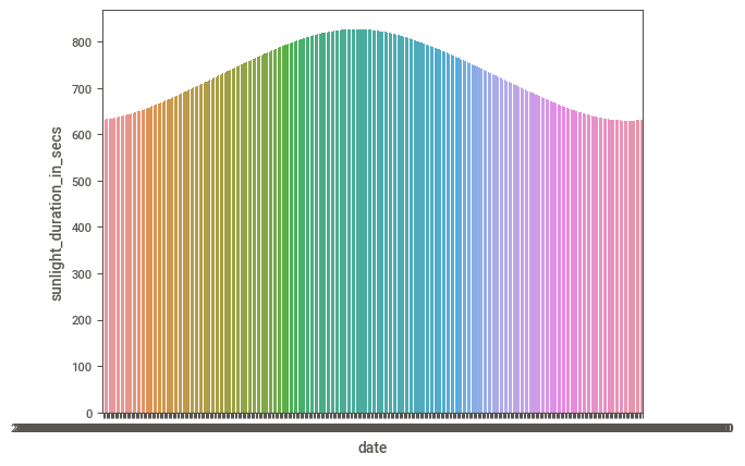

Code

# combine with target data
merged_with_external = target_data.merge(external_weather_df_selected, on='date')
assert merged_with_external.isnull().sum().sum() == 0
merged_with_external

	date	wind_power	solar_power	month	temp	dew	humidity	precip	wind_speed	winddir	visibility	solarradiation	solarenergy	uvindex	sunlight_duration_in_secs
0	2022-01-01	79.75	527.55	1	19.4	16.4	82.8	15.9	7.638889	55.0	10.2	127.7	11.2	6	631.716667
1	2022-01-02	79.75	762.18	1	20.6	18.0	85.5	3.1	9.638889	106.2	9.9	103.9	9.0	4	632.133333
2	2022-01-03	79.75	1343.82	1	18.2	13.9	76.5	0.0	6.722222	298.7	7.4	175.2	15.2	7	632.566667
3	2022-01-04	79.75	1469.36	1	16.9	9.4	61.6	0.0	9.722222	304.2	10.3	183.5	15.9	7	633.050000
4	2022-01-05	79.75	1588.27	1	15.3	4.7	49.4	0.0	9.250000	301.1	11.5	190.6	16.5	7	633.550000
...	...	...	...	...	...	...	...	...	...	...	...	...	...	...	...
360	2022-12-27	120.22	1132.27	12	19.6	14.1	70.7	0.3	4.777778	198.7	8.3	157.1	13.5	6	630.150000
361	2022-12-28	926.98	1395.73	12	17.6	10.4	63.1	0.1	12.833333	306.0	9.9	127.9	10.9	6	630.366667
362	2022-12-29	462.69	1307.64	12	18.0	11.7	67.4	0.0	10.222222	310.2	8.4	163.2	14.0	6	630.633333
363	2022-12-30	273.46	746.64	12	18.1	11.4	65.2	0.0	7.138889	305.8	10.1	123.2	10.7	5	630.916667
364	2022-12-31	170.90	865.91	12	18.3	11.9	66.5	0.1	6.611111	304.3	10.1	141.8	12.0	6	631.250000

365 rows × 15 columns

Code

analyze_report = sv.analyze([merged_with_external,'Wind Power Report'], 'wind_power')
filepath = 'reports/Extra_Features_wind_power_external_data.html'
analyze_report.show_html(filepath=filepath, layout='vertical', open_browser=False)
display(Markdown(f'**To view the report, [CLICK HERE]("{filepath}")**'))

Done! Use 'show' commands to display/save.   |██████████| [100%]   00:01 -> (00:00 left)

Report reports/Extra_Features_wind_power_external_data.html was generated.

To view the report, CLICK HERE

Code


analyze_report = sv.analyze([merged_with_external,'Solar Power Report'], 'solar_power')
filepath = 'reports/Extra_Features_solar_power_external_data.html'
analyze_report.show_html(filepath=filepath, layout='vertical', open_browser=False)
display(Markdown(f'**To view the report, [CLICK HERE]("{filepath}")**'))

Done! Use 'show' commands to display/save.   |██████████| [100%]   00:01 -> (00:00 left)

Report reports/Extra_Features_solar_power_external_data.html was generated.

To view the report, CLICK HERE